CA 7. FrequencyDomainAnalysis
Last Edit: 3/23/26
Network function, Transfer function #
Under Zero Initial Condition, the Network function is being defined as the ratio between input and output Laplace Transform
$$ T(s) = \frac{Y(s)}{X(s)} $$
This function can be extract into two parts, Natural Poles and Forced Poles
- Natural Poles: Natural Response due to poles of $T(s)$
- Forced Poles: Forced Response due to poles of $X(s)$
Observations #
- Stable Circuit: If a circuit’s Natural Response dies down to zero as time pass, then it’s a Stable Circuit
- This is equivalent to all the poles of $T(s)$ is on the Left-Half Plane of S-domain
- This is because $p = \sigma + j\omega$ is equivalent to $e^{pt} = e^{\sigma t}e^{j\omega t}$ in time domain, thus only a negative real part make this to zero eventually
Forced Response & Steady-State #
If the input signal $X(s)$’s poles is also on the left-half plane, then its Forced Response will also goes to zero
- Otherwise, this will form a Steady-State Response for those Forced Poles
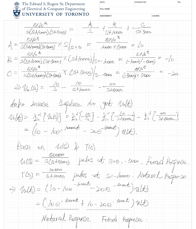
Ex. Find the Zero-State Response for RC circuit #
Transfer Function #
One-port Network #
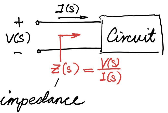
This Port’s Transfer Function is normally a Impedance, as there’s only one port, thus no transfer inside, instead all we get is a element by itself
Two-port Network #
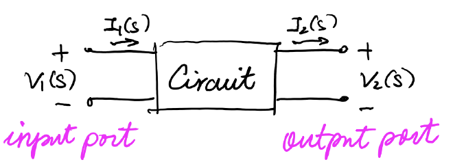
For Two-port Network, there’s an input and an output, based on the type for in and output, there could be four types of Transfer Function
- Voltage Transfer Function: $T_V(s) = \frac{V_2(s)}{V_1(s)}$
- Current Transfer Function: $T_I(s) = \frac{I_2(s)}{I_1(s)}$
- Transfer Admittance: $T_Y(s) = \frac{I_2(s)}{V_1(s)}$
- Transfer Impedance: $T_Z(s) = \frac{V_2(s)}{I_1(s)}$
Forward and Reverse Transfer Function #
Forward Transfer Function #
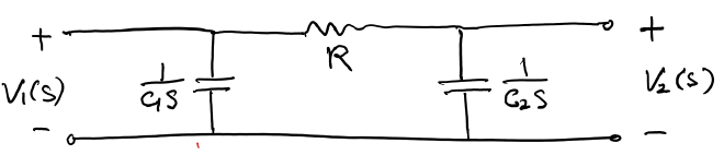
If we use $v_1(s)$ as input, then $C_1$ is neglectable in this case, what’s remaining is then only a series circuit between R and C
$$ T(s) = \frac{V_2(s)}{V_1(s)} = \frac{\frac{1}{C_2 s}}{R + \frac{1}{C_2 s}} = \frac{1/RC_2}{s + 1/RC_2} $$
Reverse Transfer Function #
Now we take $v_2(s)$ as the input, then $C_2$ is being discarded, thus
$$ T’(s) = \frac{\frac{1}{C_1s}}{R + \frac{1}{C_1s}} = \frac{1/RC_1}{s + 1/RC_1} $$
Examples of Transfer Functions #
Voltage Divider Circuit #
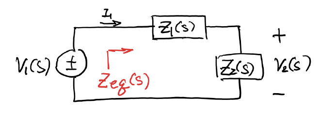
Its Voltage Transfer Function is: $T_V(s) = \frac{V_2(s)}{V_1(s)} = \frac{Z_2}{Z_1 + Z_2}$
Its Driving Point Admittance is then: $Z_{eq} = Z_1 + Z_2$
Current Divider Circuit #
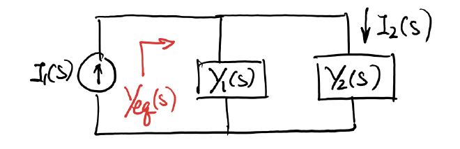
Its Current Transfer Function is $T_I(s) = \frac{I_2(s)}{I_1(s)} = \frac{Y_2}{Y_1 + Y_2}$
Its Driving-Point Admittance is $Y_{eq} = Y_1 + Y_2$
Op-amp Circuits #
There’s a lot kind of Op-amp, here we only analysis Inverting and Non-Inverting ones, but the key to analysis both of them is by Virtual Short that $(V_p=V_n, i_p=i_n=0)$
Inverting Amplifier #
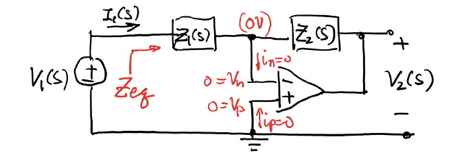
Known the closed gain for Inverting Amplifier is $T_V(s) = \frac{V_2(s)}{V_1(s)} = -\frac{Z_2}{Z_1}$
Whereas the Driving Impedance is $Z_{eq} = Z_1$
Non-Inverting Amplifier #
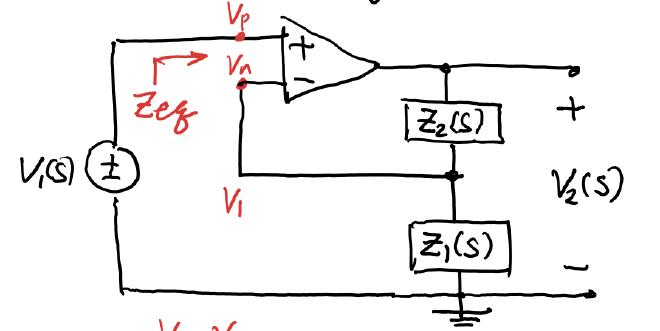
Its Transfer function is $V_1 = \frac{Z_1}{Z_1 + Z_2} V_2 \implies T_V(s) = \frac{Z_1 + Z_2}{Z_1} = 1 + \frac{Z_2}{Z_1}$
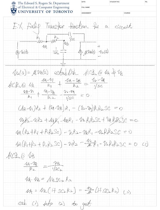
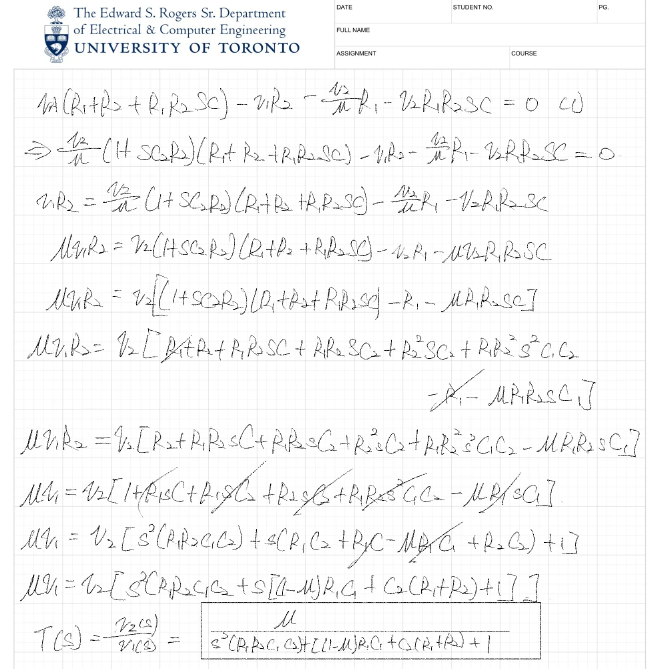
Ex. Finding Transfer Function for a Circuit #
Cascade Connection #
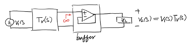
Known that a Two-port Network has the Transfer Function of $V_2(s) = T_V(s) V_1(s)$, however, this is under a open circuit configuration, if there’s a Load on the output port, it will created a divider port then
$$ V_2(s) = \underbrace{V_1(s) T_V(s)}{\text{Open Response}} \times \underbrace{\frac{Z_L}{Z_T + Z_L}}{\text{Divider Factor}} $$
This can be solved by adding a Buffer
Impulse Response, Convolution #
Definition of Impulse Function #
Impulse function has the following property
- When $t\neq 0$, $\delta(t)=0$
- Integral containing origin is always 1
Sifting Property of Impulse Function #
Impulse function can sifting a point’s value of a function at given time $t_0$
$$ \int_{-\infty}^{\infty} f(t) \delta(t-t_0) dt = f(t_0) $$
Laplace Transform of Impulse Function #
$$ D(s) = \mathcal{L}{\delta(t)} = \int_0^\infty \delta(t) e^{-st} dt=1 $$
Notice this integral is just the Sifting of function $e^{-st}$ at $t=0$, thus is equal to one
Thus we can also get $\mathcal{L}^{-1}{1} = \delta(t)$
Impulse response of a circuit #
Known in a circuit, with $\delta (t)$ as the input, the output $h(t)$ shall be the Impulse Response
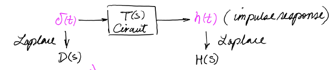
Then take both side for Laplace, we get the two S-domain function $D(s)$ and $H(s)$, notice $\mathcal L{\delta (t)} = D(s)=1$, thus we have the output as
$$ H(s) = T(s) \cdot D(s)=T(s)\cdot 1\Rightarrow H(s)=T(s) $$
Circuit response in S-domain #
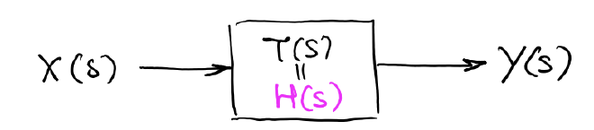
Based on the property $H(s)=T(s)$, we get $Y(s) = T(s)X(s) = H(s)X(s)$
Circuit response in Time-domain #
Taking the Inverse Laplace on both side to get
$$ y(t) = \mathcal{L}^{-1}{Y(s)} = \mathcal{L}^{-1}{H(s)X(s)} $$
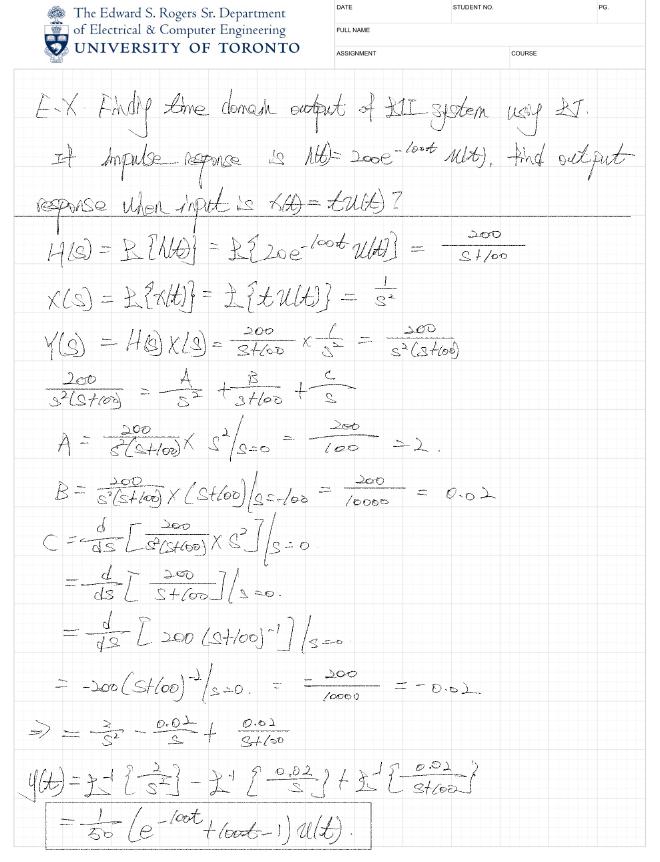
Ex. Finding the Time Domain output of LTI System using Laplace Transform #
Direct time-domain solution #
This part contains a derivation, and its final claim is
$$ Y(s) = H(s)X(s) \iff y(t) = h(t) * x(t) $$
Convolution Integral #
$$ h(t) * x(t) = \int_{0}^{t} h(t-\tau) x(\tau) d\tau $$
Property of convolution #
- Commutative: $f(t) * g(t) = g(t) * f(t)$
- Associative: $f(t) * [g(t) * w(t)] = [f(t) * g(t)] * w(t)$
- Distributive: $f(t) * [g(t) + w(t)] = [f(t) * g(t)] + [f(t) * w(t)]$
- Convolution with an impulse: $f(t) * \delta(t-t_0) = f(t-t_0)$
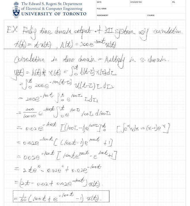
Ex. Finding the time domain output of LTI System using Convolution #
The meaning of convolution #
Result of convolution is an addition of weighted function sampled points
Step Response #
The $u(t)$ is a kind of classic step function
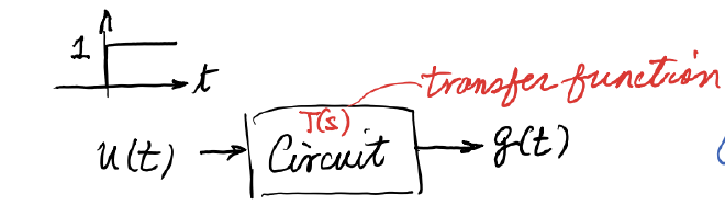
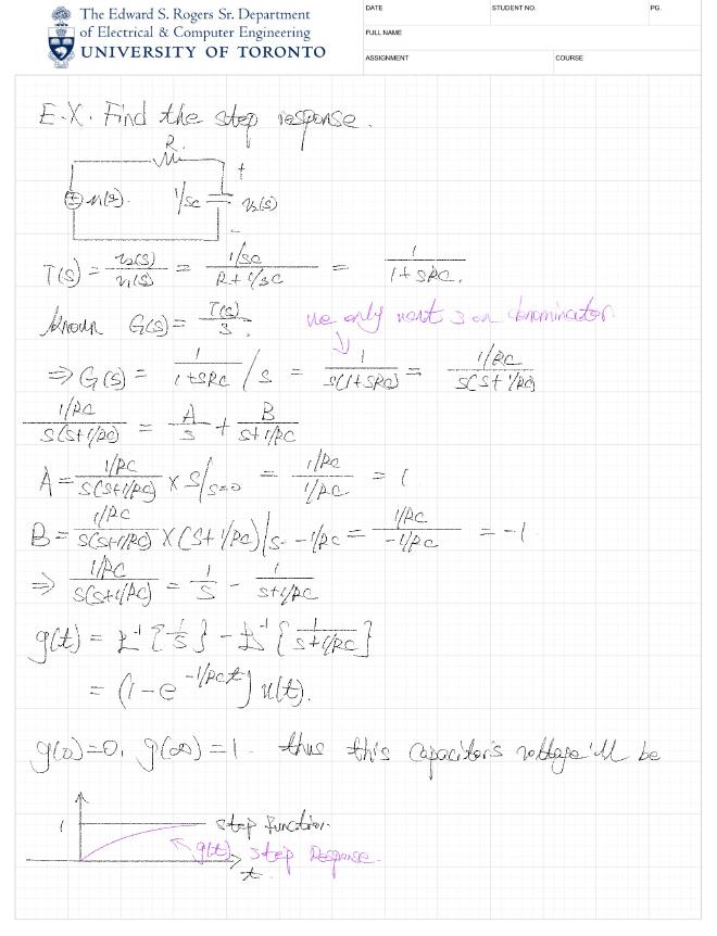
$$ G(s) = T(s) \cdot \mathcal{L}{u(t)} = T(s) \cdot \frac{1}{s} $$
Known that $T(s)$ is normally a fraction with Poles $p_1,p_2,\dots,p_n$m, that can be extract into
$$ G(s) = \frac{k_0}{s} + \frac{k_1}{s-p_1} + \dots + \frac{k_n}{s-p_n} $$
Taking the inverse Laplace Transform to get
$$ g(t) = k_0 u(t) + (k_1 e^{p_1 t} + \dots + k_n e^{p_n t}) u(t) $$
This Time domain output contains two parts, Forced Response and Natural Response
- Forced Response: $k_0 u(t)$, caused by the input signal
- Natural Response: $(k_1 e^{p_1 t} + \dots + k_n e^{p_n t}) u(t)$, determined by the poles of Transfer Function
Stable System #
For a Stable System, the Natural Response will decay to zero as time passes, so that means as time $t\rightarrow \infty$, $g(\infty)\rightarrow k_0$
And $k_0$ can be found using the Cover-up Algorithm $k_0 = s G(s) \big|{s=0} = T(s) \big|{s=0} = T(0)$, thus eventually the Step Response can be represented by
$$ g(t) = T(0) u(t) + (k_1 e^{p_1 t} + \dots + k_n e^{p_n t}) u(t) $$
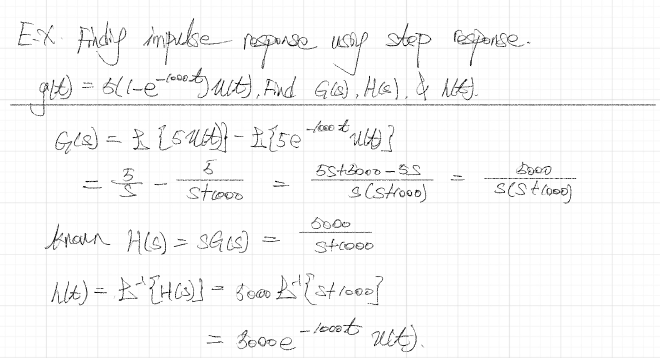
Relationship between Step response and Impulse response #
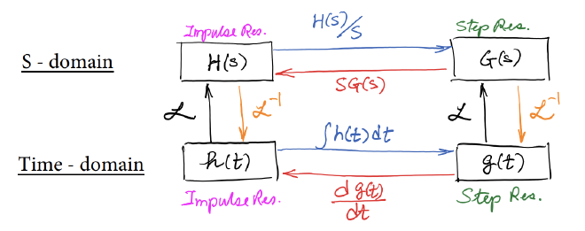
By this relationship, we can get that, if we want the Impulse Response $h(t)$ of the System which can reveal the behavior of the System, we can
- Start with a Step Function input to get the Step Response of the System
- Then use a Differentiator Circuit to get the Impulse Response $h(t)$
Ex. Find the Step Response #
Ex. #
Sinusoidal Response #
Here we are trying to analysis when the input is a Sinusoidal Signal, in the form of $x(t) = X_A \cos(\omega t + \phi)$, base on the Laplace Transform pair, we can get $X(s)$
$$ X(s) = X_A \left[ \frac{s \cos \phi - \omega \sin \phi}{(s - j\omega)(s + j\omega)} \right] $$
Notice the poles are $(s - j\omega)(s + j\omega)$ on Complex Plane
Recall the Response contains Forced Poles and natural Poles
- Forced Poles: $s = j\omega$ and $s = -j\omega$, in the form of $\frac{k}{s - j\omega} + \frac{k^*}{s + j\omega}$, taking the Inverse Lapalce will give us $y(t) = k e^{j\omega t} + k^* e^{-j\omega t}$
- Natural Poles: Due to the System itself
- Steady-State Response: When Natural Response decay to zero, then we get
$$ y_{ss}(t) = k e^{j\omega t} + k^* e^{-j\omega t} $$
Then we shall we Cover-up Algorithm to calculate $k$, that will be $k = (s - j\omega) Y(s) \big|_{s = j\omega}$, and the result will be
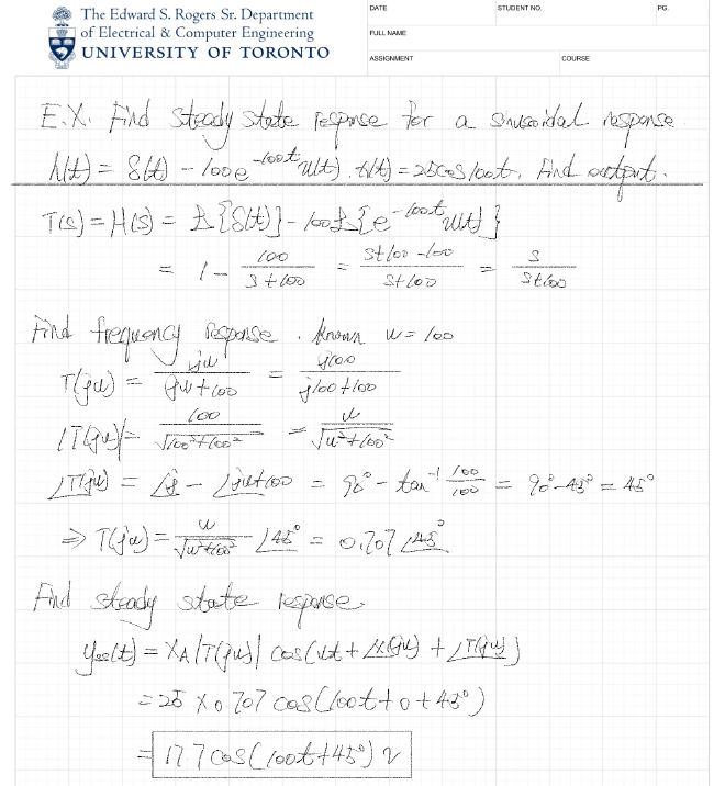
$$ y_{ss}(t) = X_A |T(j\omega)| \cos(\omega t + \phi + \theta) $$
- $X_A |T(j\omega)|$, Amplitude: Determine by Input Amplitude and System Gain
- $\phi + \theta$, Phase Angle: Determine by Input Phase and System Shifting
Ex. #
Frequency Response #
Recall the Transfer Function, with input as Various Frequency Components, the Transfer Function contains Amplitude $|T(j\omega)|$ and Phase Change $\angle T(j\omega)$ two parts
What this Transfer Function does is called the Frequency Response which is a “profile” that capture how circuit “process” signal component to different frequencies
Low Pass Filter #
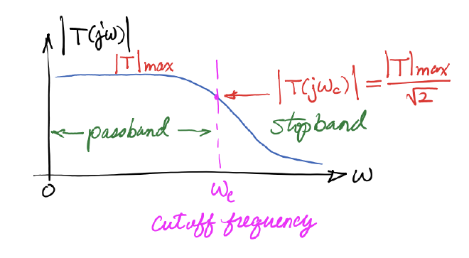
By setting a Cut Off Frequency $\omega_0$, we set up this Low Pass Filter, as this is not an Ideal LPF, we set up the frequency out of the band with a decay model
Different Filter will have there own passband Area
- Low-pass:$[0, \omega_c]$
- High-pass:$[\omega_c, \infty)$
- Band-pass:$[\omega_{c1}, \omega_{c2}$
- Band-stop: $[0, \omega_{c1}] & [\omega_{c2}, \infty)$
The Bode Diagrams #
There’s two kind of Bode Diagrams, Magnitude Plot and Phase Plot, they both have horizontal unit of frequency, and with different Vertigo Components
- Magnitude Plot: $20 \log_{10} |T(j\omega)| \text{ decibel (dB)}$, use Decibel
- Phase Plot: $\angle T(j\omega) \text{ degree}$, use Angle
Cascaded Systems #
The overall Transfer Function is the multiplication of all Transfer Functions, in the form
$$ T(j\omega) = T_1(j\omega) \times T_2(j\omega) \times \dots \times T_n(j\omega) $$
Advantage of dB Scale #
dB scale is a good way to compactly express both very large and very small values
First-order Low Pass response #
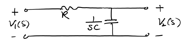
Given a RC circuit, the Voltage Transfer Function will be given as
$$ T(s) = \frac{V_2(s)}{V_1(s)} = \frac{1/sC}{R + 1/sC}= \frac{1}{1 + sRC} $$
General form of First-order low pass response #
Known the General form of First-order low pass response is $T(s) = \frac{K}{\alpha + s}$
- $s$: Complex Frequency
- $\alpha$: Poles, Cut off Frequency
- $K$: Gain Coefficient
Frequency Response of First order low pass response #
If the only thing we care is how circuit deal with frequencies, then we can simplify the term $s = \sigma + j\omega$ into $s=j\omega$, which is the Frequency Response of the system, now we get
$$ T(j\omega) = \frac{K/\alpha}{1 + j\omega/\alpha} = \frac{T(0)}{1 + j\omega/\alpha} $$
Bode Plot of the Magnitude #
Start with the Transfer Function $T(j\omega) = \frac{K}{\alpha + j\omega}$, its Amplitude shall be the mod $|T(j\omega)| = \frac{|K|}{\sqrt{\alpha^2 + \omega^2}}$, then change into $|T(j\omega)| = \frac{|T(0)|}{\sqrt{1 + (\omega/\alpha)^2}}$
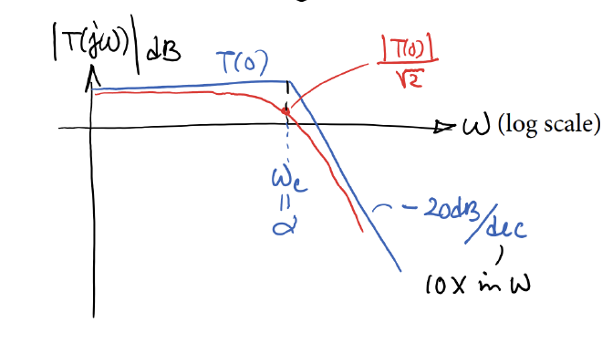
There’s three important region on this Graph
- $|T(j\omega)|_{\omega=0}$: The DC term, is equal to $|T(0)|$
- $|T(j\omega)|_{\omega=\alpha}$: At the cut off frequency, is equal to $\frac{|T(0)|}{\sqrt{2}}$
- $|T(j\omega)|_{\omega=high~\omega}$: At the region of cut off frequency, is equal to $\frac{|K|}{\omega}$
For region larger than the cut off frequency, it is followed by the equation
$$ 20\log |T(j\omega)| = |K|_{\text{dB}} - 20\log\omega $$
this was approached by taking $log$ on both side of equation
Plot of the phase angle #
Also start with $T(j\omega) = \frac{K}{\alpha + j\omega}$, then overall phase is $\angle T(j\omega) = \angle K - \arctan(\omega/\alpha)$, we can also analysis this overall phase under three frequencies
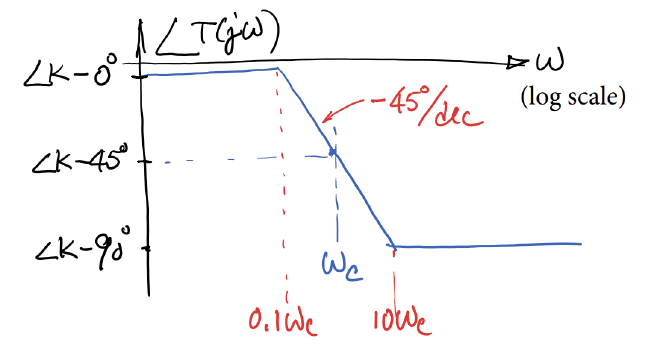
- $T(j\omega)|_{\omega=0}$: If $K$ is $+ve$, then its 0, else is $\pm 180$
- $T(j\omega)|_{\omega=\alpha}$: Phase is $\angle K - 45^{\circ}$
- $T(j\omega)|_{\omega\rightarrow \infty}$: Phase is $\angle K - 90^{\circ}$
Current Interpretation #
Recall the RC circuit,
- At Low Frequency, the Impedance $\frac{1}{j\omega C}$ is very large that it’s an open-circuit, thus $V_{out} \approx V_{in}$, $T(j\omega) \approx 1$, $\angle T(j\omega) = 0^{\circ}$
- At High Frequency, Impedance is small that is a short circuit, $T(j\omega) \approx \frac{1}{j\omega RC}$, $V_{out} \to 0$, $\angle T(j\omega) = 90^{\circ}$
Bandwidth (BW) #
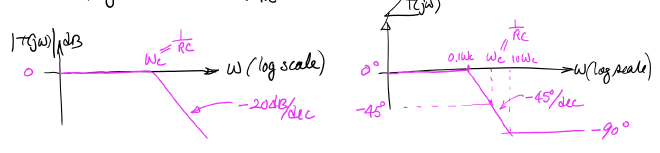
For the First Order Low Filter $T(j\omega) = \frac{T_o}{1 + j\omega/\omega_c}$, its Bode plot is
Whereas $T_0$ is the DC gain and $\omega_c$ is the Corner Frequency (AKA Bandwidth, Cut off Frequency, 3dB Frequency)
It’s called 3dB frequency because it’s 3dB lower than $T_0$
Gain-Bandwidth Product (GBW) #
This means that in a given First Order System, the product of gain and BW is a constant
Op Amp’s Bandwidth #
Based on the Gain-Bandwidth Product, we can get the Op Amp’s gain and Bandwidth once we know the other
Open-loop #
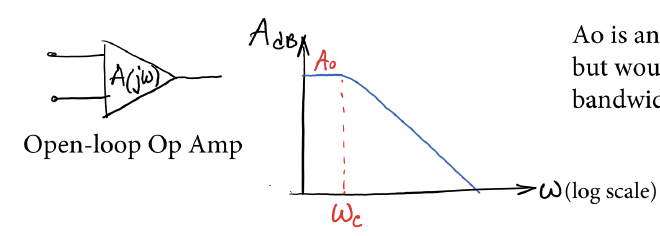
Open Loop Op amp has high gains, with $A_0=10^5-10^6$, this makes it’s $\omega_c$ really small
Closed-loop #
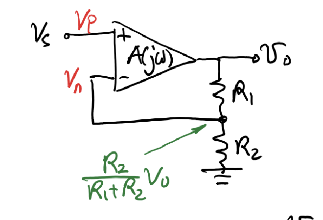
Known that the feedback coefficient is $\beta = \frac{R_2}{R_1+R_2}$, thus we can get the closed-loop gain from the formula $V_o = A(j\omega)(V_p - V_n)$
$$ \text{Closed-loop gain} = \frac{A(j\omega)}{1 + \beta A(j\omega)} $$
Now sub in the formula for First order low filter $A(j\omega) = \frac{A_o}{1 + j\omega/\omega_c}$ to get
- DC gain: $T_0=\frac{A_o}{1 + \beta A_o}$
- Cut off Frequency: $\omega_c(1 + \beta A_o)$
now we can get the new GBW formula as
$$ \text{GBW}_{closed} = \left( \frac{A_o}{1 + \beta A_o} \right) \times \left( \omega_c(1 + \beta A_o) \right) = A_o \omega_c $$
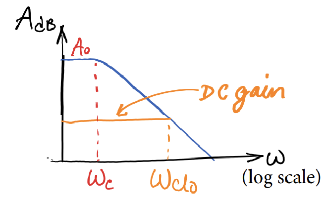
The blue line is the Frequency Response for the open loop gain, it’s also the limit of the op amp, whereas the orange one $\omega_{clo}$ is the closed loop gain in which, 1. manually decrease the amplitude, 2. but having a widther bandwidth
First-order high-pass response #
The Standard form of First-order high-pass response is
$$ T(s) = \frac{Ks}{s + \alpha} = \frac{Ks/\alpha}{1 + s/\alpha} \quad (\alpha > 0) $$
- $\alpha$ : Cut off frequency ($\omega_c$)
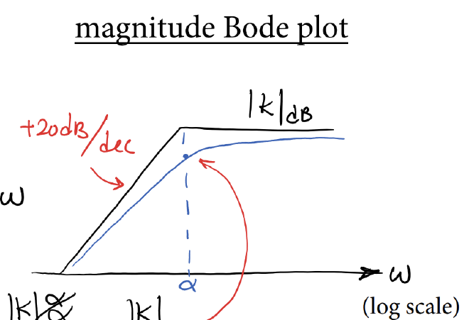
Magnitude Response #
Taking the mod of the Transfer function to get
$$ |T(j\omega)| = \frac{|K|\omega}{\sqrt{\alpha^2 + \omega^2}} = \frac{|K|\omega/\alpha}{\sqrt{1 + (\omega/\alpha)^2}} $$
- $\omega \ll \alpha$: $|T(j\omega)|= \frac{|K|\omega}{\alpha}$, under log scale, it’s increasing with the slope of $+20\text{dB/dec}$
- $\omega \gg \alpha$: $|T(j\omega)|=|K|$, the magnitude is approaching constant $K$
Phase Response #
Taking the phase of the Transfer function to get
$$ \angle T(j\omega) = \angle K + 90^\circ - \tan^{-1}(\frac{\omega}{\alpha}) $$
- $\omega = 0$: $\angle T(j\omega) =\angle K + 90^\circ$
- $\omega = \alpha$: $\angle T(j\omega) =\angle K + 45^\circ$
- $\omega \to \infty$: $\angle T(j\omega) =\angle K + 90^\circ - 90^\circ = \angle K$
Frequency Response #
By letting $s=j\omega$, we get the Frequency Response as
$$ T(j\omega) = \frac{j\omega K}{\alpha + j\omega} $$
High-pass circuit example #
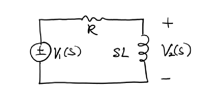
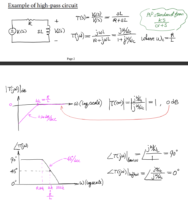
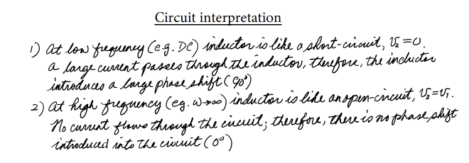
High-pass and Low-pass cascade #
The overall system is formed by a series connection of High-pass and Low-pass filter
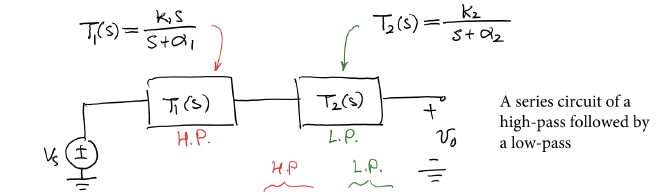
Thus we can get the overall Transfer function as the multiplication of two functions
$$ T(s) = T_1(s) \cdot T_2(s) = \frac{K_1 s}{s + \alpha_1} \cdot \frac{K_2}{s + \alpha_2} $$
Whereas its Frequency response is
$$ T(j\omega) = \frac{K_1 j\omega}{j\omega + \alpha_1} \cdot \frac{K_2}{j\omega + \alpha_2} $$
Magnitude Response of the Cascade Transfer function #
Starting with the low frequency:
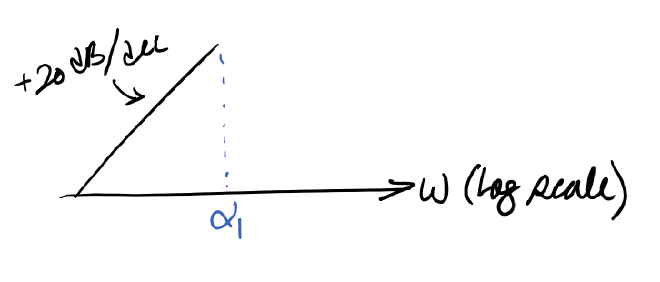
- ****$\omega \ll \alpha_1$: $|T(j\omega)|=\frac{|K_1|\omega}{\alpha_1} \cdot \frac{|K_2|}{\alpha_2}$, $|T(j\omega)|{\text{dB}} = \left| \frac{K_1 K_2}{\alpha_1 \alpha_2} \right|{\text{dB}} + 20 \log \omega$
Then the high frequency:
- $\omega \gg \alpha_2$: $|T(j\omega)|=\frac{|K_1|\omega}{\omega} \cdot \frac{|K_2|}{\omega} = \frac{|K_1 K_2|}{\omega}$, $|T(j\omega)|{\text{dB}} = |K_1 K_2|{\text{dB}} - 20 \log \omega$
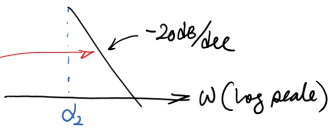
Lastly the band pass region $\alpha_1 \ll \omega \ll \alpha_2$:
- $T_1(j\omega)\rightarrow \frac{|K_1|\omega}{\omega} = |K_1|$
- $T_2(j\omega)\rightarrow \frac{|K_2|}{\alpha_2}$
Thus the overall Magnitude response is
$$ |T(j\omega)| \to \frac{|K_1 K_2|}{\alpha_2},\quad G = |K_1 K_2|{\text{dB}} - |\alpha_2|{\text{dB}} $$
Circuit Realization of Band-pass filter #
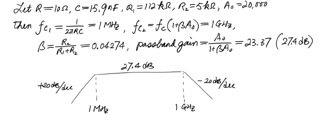
The series connection of a RC circuit and Op Amp forms a Band-pass filter
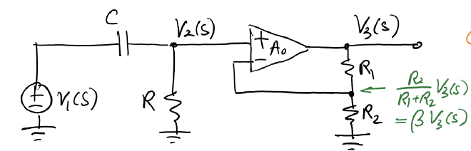
Whereas the High-pass part is the RC filter, and low-pass is the Non-inverting Amplifier, thus the overall Transfer function is
$$ T(s) = T_1(s) \cdot T_2(s) $$
High-pass part #
- Transfer function: $T_1(s) = \frac{R}{R + \frac{1}{sC}} = \frac{s}{s + \frac{1}{RC}}$
- Frequency Response: $T_1(j\omega) = \frac{j\omega}{\frac{1}{RC} + j\omega}$
- Cut-off Frequency: $f_{c_1} = \frac{\omega_{c_1}}{2\pi} = \frac{1}{2\pi RC}$
Low-pass part #
- Frequency Response: $T_2(j\omega) = \frac{\text{DC gain}}{1 + j\omega / \omega_{cl_0}} = \frac{A_0 / (1 + \beta A_0)}{1 + j\omega / (\omega_c(1 + \beta A_0))}$
- Cut-off Frequency (Angular): $\omega_{c_2} = \omega_c(1 + \beta A_0)$
- Cut-off Frequency: $f_{c_2} = \frac{\omega_{c_2}}{2\pi} = f_c(1 + \beta A_0)$
Thus the overall Transfer Function (Frequency Response) is then
$$ T(j\omega) = T_1(j\omega) T_2(j\omega) = \frac{j\omega}{\frac{1}{RC} + j\omega} \times \frac{A_0 / (1 + \beta A_0)}{1 + j\omega / (\omega_c (1 + \beta A_0))} $$
When the whole system is in the band-pass region ($\frac{1}{RC} \ll \omega \ll \omega_c(1 + \beta A_0)$), this becomes
$$ |T(j\omega)|_{\text{mid-range}} \approx 1 \times \frac{A_0}{1 + \beta A_0} = \text{Passband Gain} $$
Ex. Band-pass Filter Example #
Band-stop Response #
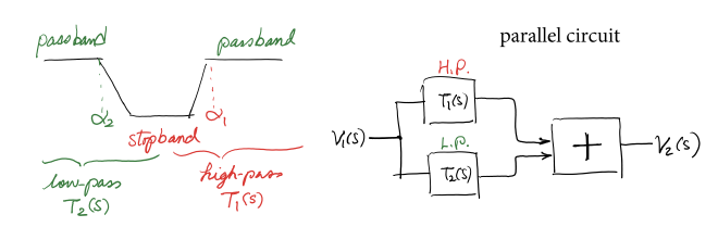
Band-stop response is a parallel connection for a High-pass and Low-pass filter, and the overall Transfer function becomes
$$ T(s) = T_1(s) + T_2(s) $$
Notice: Series Cascade is multiplication, Parallel Cascade is addition
We can also get the Frequency response and the Magnitude response
$$ T(j\omega) = \frac{j\omega K_1}{\alpha_1 + j\omega} + \frac{K_2}{\alpha_2 + j\omega},\quad |T(j\omega)| = \frac{\omega K_1}{\sqrt{\alpha_1^2 + \omega^2}} + \frac{K_2}{\sqrt{\alpha_2^2 + \omega^2}} $$
Then we can start analysing Transfer function under different frequencies
Staring with Low Frequency:
- $\omega \ll \alpha_2$: $|T(j\omega)| \approx |T_2(j\omega)| = \frac{K_2}{\alpha_2}$
Then is the High Frequency:
- $\omega \gg \alpha_1$: $|T(j\omega)| \approx |T_1(j\omega)| = K_1$
- Design choice, it’s suggested if we can make two band’s gain the same, in which $K_1 = \frac{K_2}{\alpha_2}$
Lastly the Mid Frequency:
- $\alpha_2 < \omega < \alpha_1$: $|T_1(j\omega)| = |T_2(j\omega)|, \quad \frac{K_1 \omega}{\alpha_1} = \frac{K_2}{\omega}, \quad \frac{K_1 \omega}{\alpha_1} = \frac{K_2}{\omega}, \quad \omega = \sqrt{\alpha_1 \alpha_2}$, thus the stopband gain is $\frac{K_1 \sqrt{\alpha_1 \alpha_2}}{\alpha_1} = K_1 \sqrt{\frac{\alpha_2}{\alpha_1}} \quad \text{or} \quad \frac{K_2}{\sqrt{\alpha_1 \alpha_2}}$
Circuit Realization for Band-stop Response #
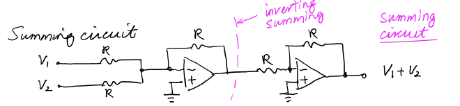
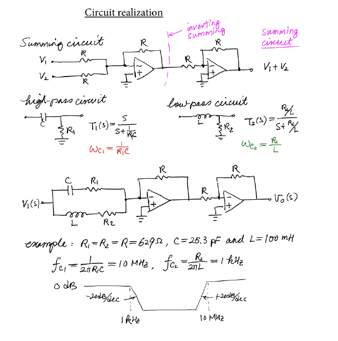
LEc 31