CA 6. Laplace
Last Edit: 3/18/26
In the previous cases, we used transfer from Time Domain to Phasor Domains to analyze circuit with Sinusoidal Steady-State, but we suggest this method is too limited. To use Laplace Transform, we are able to deal with more general ones
Laplace Transform: Transfer circuit in Time Domain into Frequency Domain (s-Domain)
- In time domain the circuit is described by Differential Equations and in Frequency Domains they are Algebraic Equations
- We first use Laplace Transfer to change it into Frequency Domain, then get the result in Frequency Domain, and change it back to time Domain using Inverse Laplace
Laplace Transform #
$$ F(s) = \mathcal{L}{f(t)} = \int_{0^{-}}^{\infty} f(t) e^{-st} dt $$
Notice the Interval of the Integral, with 0 as the lower bond, this means we assume $f(t)=0$ for all $t<0$
The Inverse Laplace Transform #
$$ f(t) = \mathcal{L}^{-1}{F(s)} = \frac{1}{2\pi j} \int_{\sigma-j\infty}^{\sigma+j\infty} F(s) e^{st} ds $$
We actually never use this, instead we follow the Laplace Transform Pairs
| 信号名称 (Signal) | 时域波形 f(t) | 复频域变换 F(s) |
|---|---|---|
| Impulse (单位冲击) | $\delta(t)$ | 1 |
| Step (阶跃函数) | $u(t)$ | $1/s$ |
| Ramp (斜坡函数) | $t u(t)$ | $1/s^2$ |
| Exponential (指数) | $e^{-\alpha t} u(t)$ | $1/(s+\alpha)$ |
| Sine (正弦) | $\sin(\beta t) u(t)$ | $\beta/(s^2+\beta^2)$ |
| Damped Sine (衰减正弦) | $e^{-\alpha t}\sin(\beta t) u(t)$ | $\beta/[(s+\alpha)^2+\beta^2]$ |
Uniqueness Property of Laplace Transform #
Laplace Transform is a one to one function that
$$ If\quad \mathcal{L}{f(t)} = F(s)\quad then\quad \mathcal{L}^{-1}{F(s)} = f(t) $$
Linearity of Laplace Transform #
$$ \mathcal{L}{a f_1(t) + b f_2(t)} = a F_1(s) + b F_2(s) $$
Integration #
Taking Integration in Time Domain equals to divided by s in s Domain
$$ \mathcal{L}{\int_0^t f(\tau) d\tau} = \frac{F(s)}{s} $$
Differentiation #
Taking differentiation in Time Domain equals to timing s and subtract initial value din s domain
$$ \mathcal{L}{\frac{df(t)}{dt}} = sF(s) - f(0^-) $$
Translation Properties #
There’s two shift for Laplace, one is shifting in Time Domain, the other is shifting in Frequency Domain
Frequency Damian Translation:
$$ \mathcal{L}{e^{\alpha t} f(t)} = F(s - \alpha) $$
Time Domain Translation
$$ \mathcal{L}{f(t-\alpha) u(t-\alpha)} = e^{-\alpha s} F(s) $$
Poles and Zeros #
For linear Circuits, the Frequency Domain $F(s)$ tends to be a Rational Fraction
$$ F(s) = K \frac{(s - z_1)(s - z_2) \dots (s - z_m)}{(s - p_1)(s - p_2) \dots (s - p_n)} $$
Whereas there are to kind of discontinuity in this Fraction, Zeros and Poles
- Zeros: When Nominator is zero
- Poles: When Denominator is zero
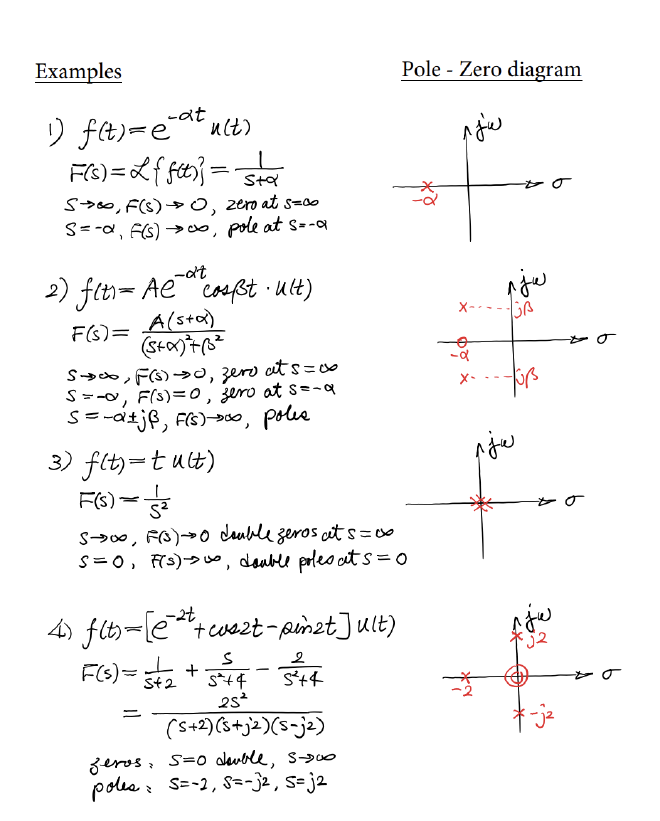
Ex. Laplace Transform and their Discontinuity #
Finding the Inverse Laplace Transform #
As indicated, most of the Laplace Function we seen will have the form of
$$ F(s) = k \frac{(s-z_1)(s-z_2) \cdots (s-z_m)}{(s-p_1)(s-p_2) \cdots (s-p_n)} $$
and there could be several cases for this function, but we need to make sure the degree of nominator must be smaller than degree of denominator to begin
Case 1: Distinct Poles #
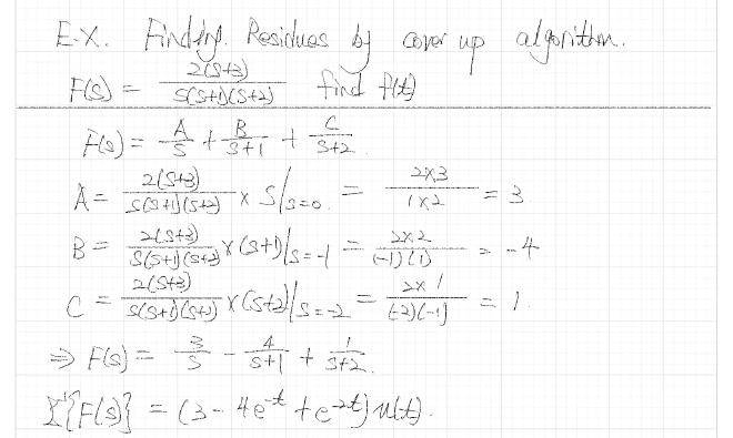
When all poles are the degree of one, thus we will have the function in the form of
$$ F(s) = \frac{k_1}{s-p_1} + \frac{k_2}{s-p_2} + \cdots + \frac{k_n}{s-p_n} $$
Where the coefficients $k_1, k_2, \dots, k_n$ here are called Residues
And Covering Up Method is what we used for finding Residues
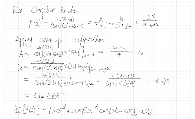
Special Case 1: Complex Roots #
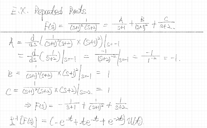
Case 2: Repeated Roots #
When one poles exist more than one times, then its a repeated root with the form
$$ F(s) = \frac{N(s)}{(s-p_1)^r (s-p_2) \cdots} $$
In this case, for that $(s-p_1)$ term, we need to expand it into r terms, which is
$$ F(s) = \frac{k_{11}}{(s-p_1)^r} + \frac{k_{12}}{(s-p_1)^{r-1}} + \cdots + \frac{k_{1r}}{s-p_1} + \text{others} $$
And in this case, we can’t use the Cover up method anymore, instead we need derivatives
$$ k_{1j} = \frac{1}{(j-1)!} \frac{d^{j-1}}{ds^{j-1}} \left[ (s-p_1)^r F(s) \right] \Bigg|_{s=p_1} $$
Special Case 2: Two Complex Double Poles #
When there’s Complex Root and there time is more than one, in the form of
$$ F(s) = \frac{K}{(s-p_j)^2(s-p_j^*)^2} = \frac{k}{(s+\alpha-j\beta)^2} + \frac{k^*}{(s+\alpha+j\beta)^2} $$
It’s Laplace Inverse in time domain will then be a sinusoid signal with time linear decay
$$ f(t) = 2|k| t e^{-\alpha t} \cos(\beta t + \theta) u(t) $$
Case 3: Improper Rational Function #
Use long division first to get the fraction in the form of a Polynomial + a Real Fraction
Laplace Circuit Analysis #
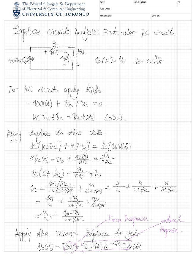
Fist Order Series RC Circuit #
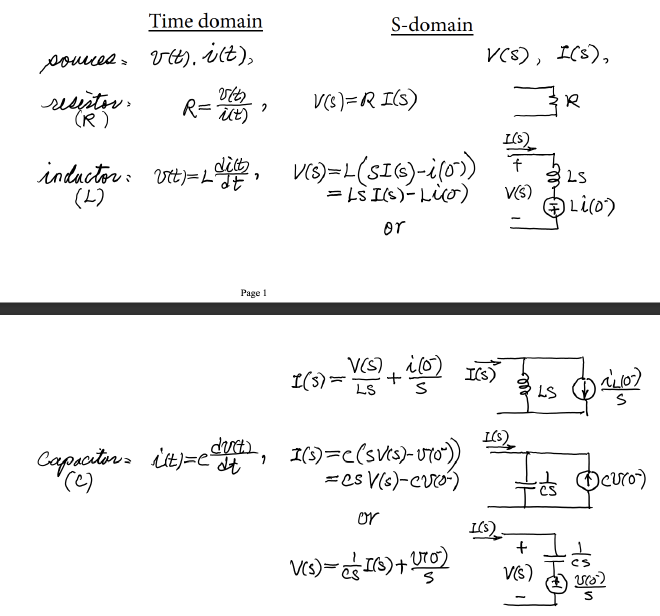
Circuit Elements in S-domain #
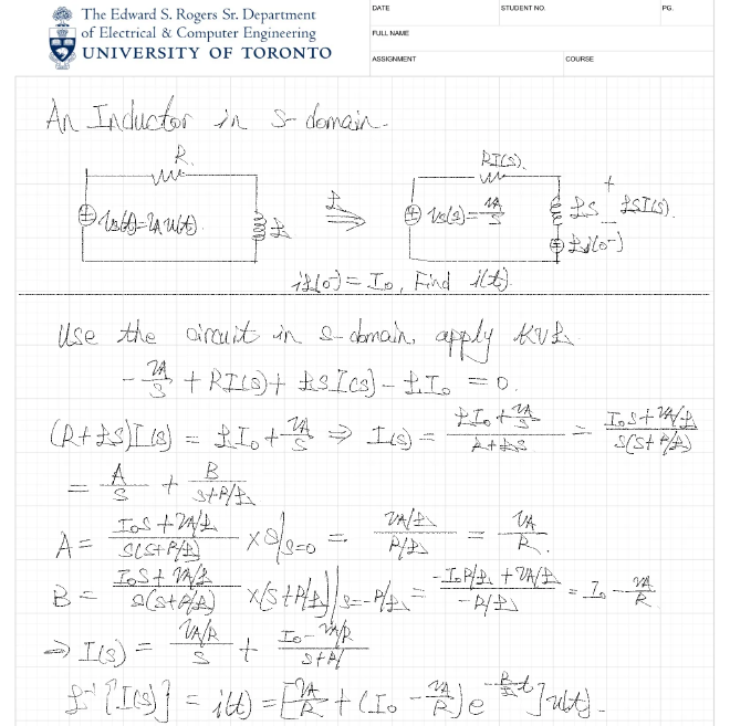
Ex. A Inductor in S-domain #
Ex. Circuit Analysis in S-domain #
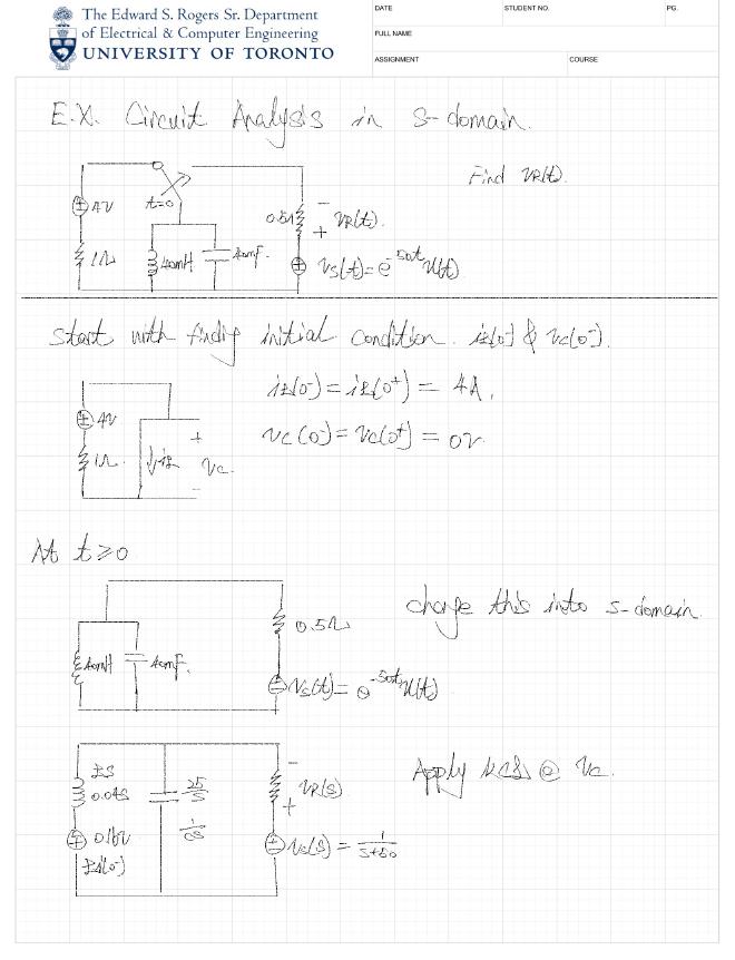
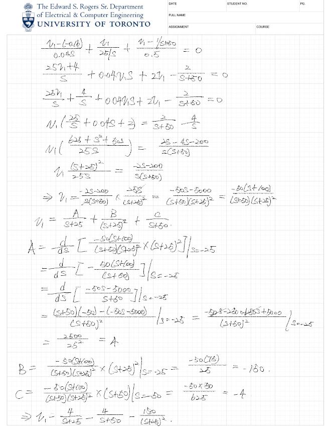
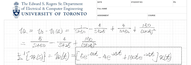
Interesting feature: combine source & switch #
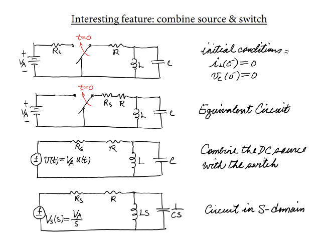
Thus in S-domain, the ODE becomes a DC circuit
Techniques applicable in S-domain #
There’s some same techniques we used in time domain that can be also apply on the S-domain
- Series and Parallel Equivalence of Impedances
- Voltage and Current division rules
- Superposition
- Nodal and Mesh Analysis
- Thevenin and Norton Equivalent Circuits
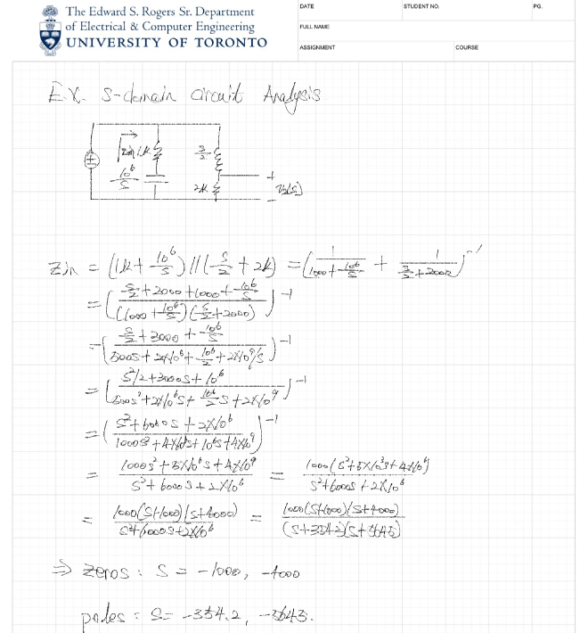
Ex. S-domain Circuit Analysis #