Last Edit 11/21/2024
正交向量Orthogonal vectors
#
正交就是垂直(perpendicular)的另一种说法
两向量正交的判据之一是其点 积\(x^Ty=y^Tx\)=0
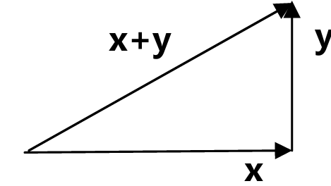
当两个向量的夹角为90度时,按照勾股定理(毕达哥拉斯定理 Pythagorean theorem)x,y满足
$$\|\mathbf{x}\|^2 + \|\mathbf{y}\|^2 = \|\mathbf{x} + \mathbf{y}\|^2 ,||\mathbf{x}\|^2 = \mathbf{x}^T \mathbf{x}$$
Orthogonal Subspaces 正交子空间
#
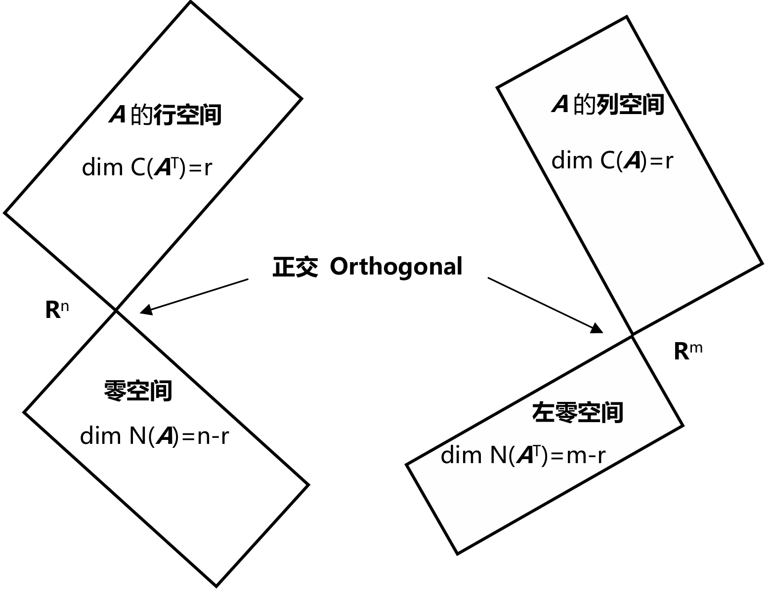
图中绘制空间成90度角,这是表示这两个空间正交
子空间S与子空间T正交,则S中的任意一个向量都和T中的任意向量正交
Nullspace is perpendicular to row space 零空间与行空间正交
#
矩阵A的行空间和它的零空间正交。若x在零空间内,则有Ax=0
$$\begin{bmatrix}
\text{row}_1 \\
\text{row}_2 \\
\vdots \\
\text{row}_m
\end{bmatrix} \times \mathbf{x} = \begin{bmatrix}
\text{row}_1 \cdot \mathbf{x} \\
\text{row}_2 \cdot \mathbf{x} \\
\vdots \\
\text{row}_m \cdot \mathbf{x}
\end{bmatrix} = \begin{bmatrix}
0 \\
0 \\
\vdots \\
0
\end{bmatrix}
$$
x与矩阵A的行向量点积都等于0,则它和矩阵A行向量的线性组合进行点积也为0,所以x与A的行空间正交
同理可以证明列空间与左零空间正交
Orthogonal complements 正交补
#
行空间和零空间不仅仅是正交,并且其维数之和等于n,我们称行空间和零空间为\(R^n\)空间内的正交补 Orthogonal complements
Orthonormal
#
如果矩阵的列向量是互相垂直的单位向量,则它们一定是线性无关的
我们将这种向量称之为标准正交(orthonormal)
$$例如\begin{bmatrix}
1 \\
0 \\
0
\end{bmatrix}
,
\begin{bmatrix}
0 \\
1\\
0
\end{bmatrix},
\begin{bmatrix}
0 \\
0 \\
1
\end{bmatrix}
还有
\begin{bmatrix}
\cos \theta \\
\sin \theta
\end{bmatrix}
,
\begin{bmatrix}
\cos \theta \\
\sin \theta
\end{bmatrix}$$
## Orthonormal Vectors 标准正交向量
$$q_i^T q_j =
\begin{cases}
0 & \text{若 } i \neq j \\
1 & \text{若 } i = j
\end{cases}$$
ATA
#
下面讨论如何求解一个无解方程组Ax=b的解
它是一个\(n\times n\)方阵,并且是对称阵\((A^TA)^T=(A^TA)\)
本章的核心内容就是当Ax=b无解的时候,求解\(A^TAx\)=\(A^Tb\)得到最优解
$$例:A = \begin{bmatrix} 1 & 1 \\ 1 & 2 \\ 1 & 5 \end{bmatrix}, \quad \text{则} \ A^T A = \begin{bmatrix} 1 & 1 & 1 \\ 1 & 2 & 5 \end{bmatrix} \begin{bmatrix} 1 & 1 \\ 1 & 2 \\ 1 & 5 \end{bmatrix} = \begin{bmatrix} 3 & 8 \\ 8 & 30 \end{bmatrix} \text{是可逆的矩阵。}
$$
$$例:A = \begin{bmatrix} 1 & 3 \\ 1 & 3 \\ 1 & 3 \end{bmatrix}, \quad \text{则} \ A^T A = \begin{bmatrix} 1 & 1 & 1 \\ 3 & 3 & 3 \end{bmatrix} \begin{bmatrix} 1 & 3 \\ 1 & 3 \\ 1 & 3 \end{bmatrix} = \begin{bmatrix} 3 & 9 \\ 9 & 27 \end{bmatrix} \text{是不可逆矩阵。}
$$
Projections in 2D 2D中的投影
#
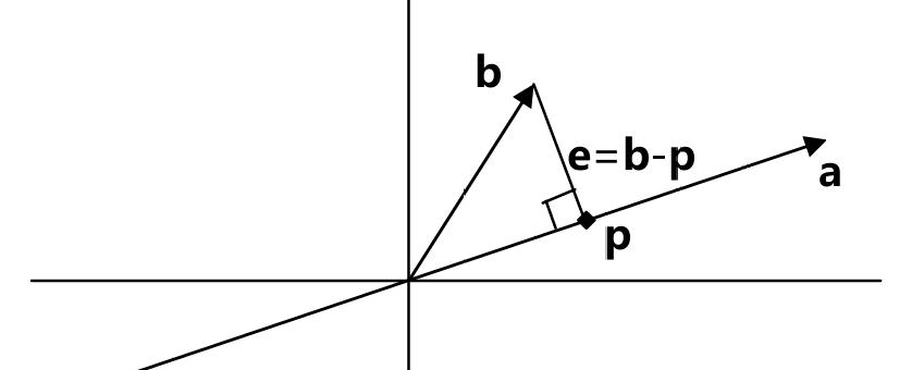
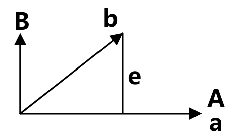
投影的几何解释便是:在向量a的方向上寻找与向量b距离最近的一 点
这个距离最近的点p就位于穿过b点并与向量a正交的直线 与向量a所在直线的交点上
则p就是b在a上的投影
如果我们将向量p视为b 的一种近似,则长度e=b-p就是这一近似的误差
于是便有方程\(a^T(b-xa)=0\)
因为向量a和b是列向量,在计算它们的点积(即内积)时,通常需要将其中一个向量转置成行向量,这样才能进行矩阵乘法并得到标量
$$\begin{equation}
x = \frac{\mathbf{a}^T \mathbf{b}}{\mathbf{a}^T \mathbf{a}}, \quad p = a x = \mathbf{a} \frac{\mathbf{a}^T \mathbf{b}}{\mathbf{a}^T \mathbf{a}}.
\end{equation}
$$
如果方程的自变量发生改变,p的改变量
如果b变为原来的2倍,则p也变为原来的2倍
而如果a变为原来的2倍, p不发生变化 (从几何角度考虑也很合理)
Projection Matrix in 2D
#
$$proj_p=Pb$$
$$\begin{equation}
p = a x = a \frac{\mathbf{a}^T \mathbf{b}}{\mathbf{a}^T \mathbf{a}}. \quad \text{则有} \quad P = \frac{\mathbf{a} \mathbf{a}^T}{\mathbf{a}^T \mathbf{a}}.
\end{equation}
$$
其分子\(aa^T\)是一个矩阵,而分母\(a^Ta\)是一个数 观察这个矩阵可知,矩阵P的列空间就是向量a所在的直线
矩阵的秩是1 (直线)
Property of projection 投影的性质
#
Symmetry 对称性
#
Apply Twice
#
如果做两次投影则有P2b=Pb,这是因为 第二次投影还在原来的位置。
因此矩阵P有如下性质:\(P^T=P,P^2=P\)
Closest vector 最短向量
#
方程Ax=b有可能无解
当出现比Unknown更多的Equations的时候,只能求解最优解
Ax一定在矩阵A的列空间之内,但是b不一定,
p是b在Colunm Space上的Projection,所以其是最优解
将问题转化为求解\(A\hat x=p\)
Closest Vector Theorem
#
Suppose V is a subspace of Rn and \(\vec x ∈ R^n\). The closest vector in V to \(\vec x\) is given by \(ProjV (\vec x )\)
In other words, \(|\text{Proj}_V(\vec{x}) - \vec{x}| \leq |\vec{v} - \vec{x}|~\text{for any } \vec{v} \in V\)
投影的方向到向量上最短的点就是其在改方向上的投影到向量的距离
Proof
#
$$\|\vec{v} - \vec{x}\|^2 = \|\vec{v} + \text{Proj}_V(\vec{x}) - \text{Proj}_V(\vec{x}) - \vec{x}\|^2 \\
= \|\vec{v} - \text{Proj}_V(\vec{x}) + \text{Proj}_V(\vec{x}) - \vec{x}\|^2$$
$$\|\vec{v} - \vec{x}\|^2 = \|\vec{v} - \vec{x}^\parallel + \vec{x}^\parallel - \vec{x}\|^2 \\
= \|\vec{v} - \vec{x}^\parallel - \vec{x}^\perp\|^2$$
$$\|\vec{v} - \vec{x}\|^2 = \|\vec{v} - \vec{x}^\parallel\|^2 + \|-\vec{x}^\perp\|^2 \\
= \|\vec{v} - \vec{x}^\parallel\|^2 + \|\vec{x}^\perp\|^2$$
可以发现\(|\vec{v} - \vec{x}|^2\)最小的值出现在\(\vec{v} = \vec{x}^\parallel\)的时候
Orthogonal projection 正交投影
#
注意Orthogonal Projection和Orthogonal Linear Transformation是完全不同的东西
之所以叫Orthogonal Projection指的是这个Projection就是最一般的情况,就是一般所理解的正交于一个Subspace的投影
在上面的\(P = A (A^T A)^{-1} A^T\)中,之所以不拆成\(P=AA^{-1}(A^T)^{-1}A^T=I\),是因为A并不是Square Matrix,即不存在Inverse
当A为Square Matrix的时候,即m=n,Input dim = Output dim,这个Projection也就变成了Identity Matrix,即将自身Project Into自己的空间
但是即使是Projecct到自己的Space,其中仍会包含Linear Transformation
Orthogonal Projection Formula 正交投影公式
#
正交投影公式是通过公式 计算一个正交的投影向量在目标子空间的投影,和Orthogonal Linear Transformation无关
对于一组Orthogonal的Basis,将Vector投影到改Space的公式为
$$\text{Proj}_V(\vec{x}) = \vec{u}_1 (\vec{u}_1 \cdot \vec{x}) + \vec{u}_2 (\vec{u}_2 \cdot \vec{x})$$
举例来说,对于一组Orthonormal Vector $$u = {\begin{bmatrix}\frac{1}{\sqrt{2}} \0 \\frac{1}{\sqrt{2}}\end{bmatrix},\begin{bmatrix}-\frac{1}{\sqrt{2}} \0 \\frac{1}{\sqrt{2}}\end{bmatrix}$$
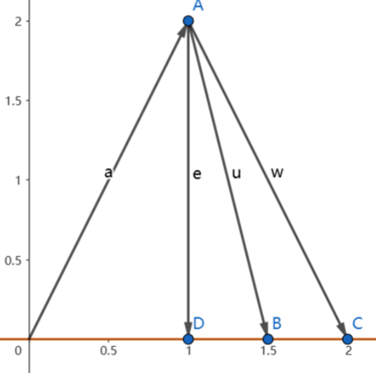
\([2,2,2]^T\)的Projection为
$$\begin{align*}
&= \begin{bmatrix}
\frac{1}{\sqrt{2}} \\
0 \\
\frac{1}{\sqrt{2}}
\end{bmatrix}
\left( \begin{bmatrix}
\frac{1}{\sqrt{2}} \\
0 \\
\frac{1}{\sqrt{2}}
\end{bmatrix} \cdot
\begin{bmatrix}
\sqrt{2} \\
0 \\
\sqrt{2}
\end{bmatrix} \right)
+
\begin{bmatrix}
-\frac{1}{\sqrt{2}} \\
0 \\
\frac{1}{\sqrt{2}}
\end{bmatrix}
\left( \begin{bmatrix}
-\frac{1}{\sqrt{2}} \\
0 \\
\frac{1}{\sqrt{2}}
\end{bmatrix} \cdot
\begin{bmatrix}
\sqrt{2} \\
0 \\
\sqrt{2}
\end{bmatrix} \right) \\
&= 2 \begin{bmatrix}
\frac{1}{\sqrt{2}} \\
0 \\
\frac{1}{\sqrt{2}}
\end{bmatrix}
=
\begin{bmatrix}
\sqrt{2} \\
0 \\
\sqrt{2}
\end{bmatrix}
\end{align*}$$
Projection Matrix 正交投影矩阵
#
正交投影矩阵,将向量正交投影到Subspace上的一个矩阵 ,A可以是任意矩阵,不是非得是Orthogonal Matrix,其和正交投影公式干的是一样的事,不过用了不同的表达方式
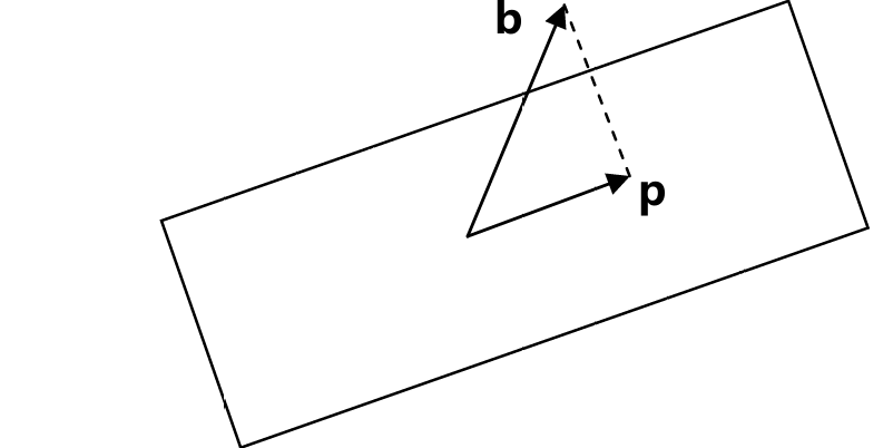
在\(R^3\)空间内,如何将向量b投影到它距离平面最近的一点p?
如果a1和a2构成了平面的一组基,则平面就是矩阵\(A=[a1,a2]\)的列空间
\(e=b-p\)是垂直于平面的
已知p在平面内,于是有\(p=\hat x_1a_1+\hat x_2a_2=A\hat x\)
而\(e=b-p=b- A\hat x\)正交于平面,因此e与\(a_1\),\(a_2\)均正交
因此可以得到:\(a_1^T(b-A\hat x )=0\)并且\(a_2^T(b-A\hat x )=0\)
因为a1和a2分别为矩阵A的列向量,即\(a1^T\)和\(a2^T\)为矩阵\(A^T\)的行向量
\(A^T(b-A\hat x)=0\)
由于\(b-A\hat x\)在于矩阵AT的零空间\(N(A^T)\)里,从上一讲讨论子空间的正交性可知,向量e与矩阵A的列空间正交,这也正是方程的意义
$$\begin{align}
\hat{x} &= (A^T A)^{-1} A^T b \\
p &= A \hat{x} = A (A^T A)^{-1} A^T b \\
P &= A (A^T A)^{-1} A^T=\frac{AA^T}{A^TA}
\end{align}$$
注意区别大小写P
对于上面的等式在dim = 1中则是\(\frac{\mathbf{a} \mathbf{a}^T}{\mathbf{a}^T \mathbf{a}}\)
投影矩阵\(P=A(A^TA)^{-1}A^T\),当它作用于向量b,相当于把b投影到矩阵A的列空间
Case when b is in column Space A
#
$$\begin{align*}
\mathbf{Pb} &= \mathbf{A}(\mathbf{A}^\top \mathbf{A})^{-1} \mathbf{A}^\top \mathbf{b} \\
&= \mathbf{A}(\mathbf{A}^\top \mathbf{A})^{-1} \mathbf{A}^\top \mathbf{Ax} \\
&= \mathbf{A}((\mathbf{A}^\top \mathbf{A})^{-1} \mathbf{A}^\top \mathbf{A}) \mathbf{x} \\
&= \mathbf{Ax} = \mathbf{b}
\end{align*}$$
Case when b orthorgal to column Space A
#
如果向量b与A的列空间正交,即向量b在矩阵A的左零空间N(A)中
在Left Null Space的意义在于\(A^Tb=0\),所以\(Pb=0\)
$$\mathbf{Pb} = \mathbf{A}(\mathbf{A}^\top \mathbf{A})^{-1} \mathbf{A}^\top \mathbf{b} = \mathbf{A}(\mathbf{A}^\top \mathbf{A})^{-1} (\mathbf{A}^\top \mathbf{b}) = \mathbf{A}(\mathbf{A}^\top \mathbf{A})^{-1} 0 = 0$$
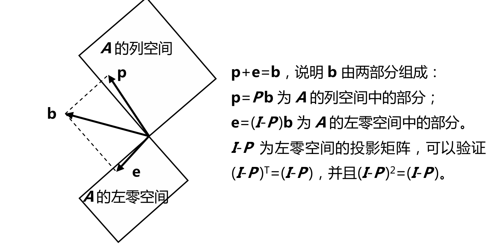
I−P 的效果 : I - P 则是从向量x中移除其在A的列空间上的分量,留下的部分即为x在A的列空间的正交补上的分量这表明I - P将向量x投影到A的列空间的正交补空间上
Orthogonal Projection Matrix in Orthogonal Basis 矩阵为正交矩阵的正交投影矩阵
#
正交矩阵的正交投影矩阵的正确读法是,当正交投影矩阵的矩阵为正交矩阵的情况下的正交投影,即改投影矩阵的A为Q的情况下,改投影将不体现“投影”的作用,而是在原空间中做Orthogonal Linear Transformation
Orthogonal Projection Matrix必须是Square Matrix
$$\mathbf{P} = \mathbf{Q} (\mathbf{Q}^\top \mathbf{Q})^{-1} \mathbf{Q}^\top$$
- 因为\\(Q^TQ=I\Rightarrow P=QQ^T\\)
如果Q为Square Matrix,则是一个投影到自身空间的Matrix,即\(P=I\),因为Q的列向量张成了整个空间,投影过程不会对向量有任何改变
就上面的例子来说,其Projection在用了Matrix后可以得到
Orthogonal Matrix 正交矩阵
#
注意这里定义的不再是投影了,而是前面提到的矩阵为正交矩阵的正交投影矩阵,是一个东西
Orthogonal Matrix 正交矩阵
#
Consider an n × n matrix A The matrix A is orthogonal if and only if \(A^TA = I\) or, equivalently, if \(A^{−1} = A^T\)
Orthogonal Matrix的Column Vector需要Norm = 1
$$\mathbf{Q} = \begin{bmatrix} 0 & 0 & 1 \\ 1 & 0 & 0 \\ 0 & 1 & 0 \end{bmatrix}, \quad
\text{则有 } \mathbf{Q}^\top = \begin{bmatrix} 0 & 1 & 0 \\ 0 & 0 & 1 \\ 1 & 0 & 0 \end{bmatrix}
$$
再比如\(\begin{bmatrix} 1 & 1 \ 1 & -1 \end{bmatrix} \text{ 并不是正交矩阵}.\)
因为其Norm为2,\(\mathbf{Q} = \frac{1}{\sqrt{2}} \begin{bmatrix} 1 & 1 \ 1 & -1 \end{bmatrix}\),调整后便可以了
一个例子便是Rotation Matrix
$$T(\vec{x}) = \begin{bmatrix}
\cos(\theta) & -\sin(\theta) \\
\sin(\theta) & \cos(\theta)
\end{bmatrix} \vec{x}$$
对于Orthogonal Matrix来说,\(Q^TQ=I\)
$$\mathbf{Q} = \begin{bmatrix} \mathbf{q}_1 & \cdots & \mathbf{q}_n \end{bmatrix}, \quad
\mathbf{Q}^\top \mathbf{Q} = \begin{bmatrix} \mathbf{q}_1^\top \\ \vdots \\ \mathbf{q}_n^\top \end{bmatrix}
\begin{bmatrix} \mathbf{q}_1 & \cdots & \mathbf{q}_n \end{bmatrix} = \mathbf{I}$$
Orthogonal transformations preserve orthogonality 角度不变性
#
Orthogonal linear transformations不仅保持向量的长度,也保持向量间的角度和orthogonality 正交性
变换前后角度不变的变换是Orthogonal transformation
Proof
#
$$||\vec x^2+\vec y^2||=||\vec x^2||+||\vec y^2||$$
需要证明\(|T(\vec{v}) + T(\vec{w})|^2 = |T(\vec{v})|^2 + |T(\vec{w})|^2\)
对于两个Orthogonal Vector \(\vec v ~& ~\vec w\),T是Linear Transformation,有
$$\|T(\vec{v}) + T(\vec{w})\|^2 = \|T(\vec{v} + \vec{w})\|^2$$
由于Orthogonal Linear Transformation preserves the norm of vector
$$\|T(\vec{v} + \vec{w})\|^2=||\vec v+\vec w||^2$$
$$||\vec v+\vec w||^2=||\vec v^2||+||\vec w||^2$$
$$||\vec v^2||+||\vec w||^2= \|T(\vec{v})\|^2 + \|T(\vec{w})\|^2$$
Orthogonal linear transformations preserves dot product 点积不变性
#
T : \(\mathbb{R}^n \to \mathbb{R}^n\) is an orthogonal transformation if and only if
$$ T(\vec{v}) \cdot T(\vec{w}) = \vec{v} \cdot \vec{w} \text{ for all } \vec{v}, \vec{w} \in \mathbb{R}^n$$
if \(\vec{u}\) and \(\vec{v}\) are orthogonal, then \(T(\vec{u})\) and \(T(\vec{v})\) are also orthogonal
变换前后dot product不变的变换就是Orthogonal Transformation
Proof
#
T : \(R^n → R^n\) is an orthogonal linear transformation
$$T(\vec{u}) \cdot T(\vec{v}) = (u_1 T(\vec{e}_1) + \dots + u_n T(\vec{e}_n)) \cdot (v_1 T(\vec{e}_1) + \dots + v_n T(\vec{e}_n))$$
根据\(q_i^T q_j = \begin{cases} 0 & \text{若 } i \neq j \1 & \text{若 } i = j \end{cases}\)
$$T(\vec{u}) \cdot T(\vec{v}) = u_1 v_1 T(\vec{e}_1) \cdot T(\vec{e}_1) + \ldots + u_n v_n T(\vec{e}_n) \cdot T(\vec{e}_n)$$
$$= u_1 v_1 \|T(\vec{e}_1)\|^2 + \ldots + u_n v_n \|T(\vec{e}_n)\|^2 \\
= u_1 v_1 + \ldots + u_n v_n
= \vec{u} \cdot \vec{v}$$
Converse statement of orthogonal linear transformation 逆命题的成立
#
if a linear map preserves orthonormality , it should preserve length and hence is an orthogonal map
Orthogonal transformations and orthonormal bases 正交基底保证正交变换
#
A linear transformation T : \(R^n → R^n\) is an orthogonal transformation if and only if the vectors \(T (\vec e_1), T(\vec e_2), . . . , T (\vec e_n)\) form an orthonormal basis for \(R^n\)
当Column Space为Orthogonal Vector的时候,Matrix为Orthogonal Transformation
Proof
#
$$\|T(\vec{x})\|^2 = \|T(x_1 \vec{e}_1 + x_2 \vec{e}_2 + x_3 \vec{e}_3)\|^2$$
$$=\|T(x_1 \vec{e}_1) + T(x_2 \vec{e}_2) + T(x_3 \vec{e}_3)\|^2 \quad (\text{by linearity of } T)$$
$$= \|T(x_1 \vec{e}_1)\|^2 + \|T(x_2 \vec{e}_2)\|^2 + \|T(x_3 \vec{e}_3)\|^2 \quad (\text{by Pythagoras})$$
$$= x_1^2 \|T(\vec{e}_1)\|^2 + x_2^2 \|T(\vec{e}_2)\|^2 + x_3^2 \|T(\vec{e}_3)\|^2 \quad (\text{by linearity of } T)$$
$$= x_1^2 + x_2^2 + x_3^2 =||\vec x||^2~(\text{since columns are length } 1)$$
$$\mathbf{Q} = \frac{1}{3} \begin{bmatrix}
1 & -2\\
2 & -1 \\
2 & 2
\end{bmatrix}, \text{ 我们可以拓展其成为正交矩阵 } \frac{1}{3} \begin{bmatrix}
1 & -2 & 2 \\
2 & -1 & -2 \\
2 & 2 & 1
\end{bmatrix}$$
Hadamard Matrix
#
$$\mathbf{Q} = \frac{1}{2} \begin{bmatrix}
1 & 1 & 1 & 1 \\
1 & -1 & 1 & -1 \\
1 & 1 & -1 & -1 \\
1 & -1 & -1 & 1
\end{bmatrix}$$
仅包含-1和1的Orthogonal Matrix
$$\text{Proj}_V(\vec{x}) = Q Q^T \vec{x} =
\begin{bmatrix}
\frac{1}{\sqrt{2}} & -\frac{1}{\sqrt{2}} \\
0 & 0 \\
\frac{1}{\sqrt{2}} & \frac{1}{\sqrt{2}}
\end{bmatrix}
\begin{bmatrix}
\frac{1}{\sqrt{2}} & 0 & \frac{1}{\sqrt{2}} \\
-\frac{1}{\sqrt{2}} & 0 & \frac{1}{\sqrt{2}}
\end{bmatrix}
\begin{bmatrix}
\sqrt{2} \\
\sqrt{2} \\
\sqrt{2}
\end{bmatrix}
=
\begin{bmatrix}
1 & 0 & 0 \\
0 & 0 & 0 \\
1 & 0 & 0
\end{bmatrix}
\begin{bmatrix}
\sqrt{2} \\
\sqrt{2} \\
\sqrt{2}
\end{bmatrix}
=
\begin{bmatrix}
\sqrt{2} \\
0 \\
\sqrt{2}
\end{bmatrix}
$$
Gram-Schmidt 施密特正交化
#
一般来说,要获得Orthogonal Matrix,先要做一步化简到该形式,这一步的名字就 Gram-Schmidt
从两个线性无关的向量a和b开始,它们张成了一个空间
我们的目标是找到两个标准正交的向量q1,q2能张成同样的空间
Schmidt给出的结论是如果 我们有一组正交基A和B,那么我们令它们除以自己的长度就得到标准正交基
$$\mathbf{q}_1 = \frac{\mathbf{A}}{\|\mathbf{A}\|}, \quad \mathbf{q}_1 = \frac{\mathbf{A}}{\|\mathbf{A}\|}
$$
当确认了一个方向后,要求出orthogonal于改方向的Vector则就是将b投影到a的方向,取B=b-p(e)
$$\mathbf{B} = \mathbf{b} - \frac{\mathbf{A}^\top \mathbf{b}}{\mathbf{A}^\top \mathbf{A}} \mathbf{A}$$
通过两边乘上\(A^T\)证明其Orthogonal性质
$$A^T\mathbf{B} = A^T(\mathbf{b} - \frac{\mathbf{A}^\top \mathbf{b}}{\mathbf{A}^\top \mathbf{A}} \mathbf{A})=0$$
Third Vector
#
$$\mathbf{q}_1 = \frac{\mathbf{A}}{\|\mathbf{A}\|}, \quad \mathbf{q}_1 = \frac{\mathbf{A}}{\|\mathbf{A}\|}\quad \mathbf{q}_3 = \frac{\mathbf{C}}{\|\mathbf{C}\|}$$
$$\mathbf{C} = \mathbf{c} - \frac{\mathbf{A}^\top \mathbf{c}}{\mathbf{A}^\top \mathbf{A}} \mathbf{A} - \frac{\mathbf{B}^\top \mathbf{c}}{\mathbf{B}^\top \mathbf{B}} \mathbf{B}
$$
ex. Two Vectors
#
$$\mathbf{a} = \begin{bmatrix} 1 \\ 1 \\ 1 \end{bmatrix}, \quad
\mathbf{b} = \begin{bmatrix} 1 \\ 0 \\ 2 \end{bmatrix}, \quad
\text{则有 } \mathbf{A} = \mathbf{a}, \quad
\mathbf{B} = \begin{bmatrix} 1 \\ 0 \\ 2 \end{bmatrix} - \frac{3}{3} \begin{bmatrix} 1 \\ 1 \\ 1 \end{bmatrix} = \begin{bmatrix} 0 \\ -1 \\ 1 \end{bmatrix}$$
- 则有Orthonormal Matrix Q
$$\mathbf{Q} = \begin{bmatrix} \mathbf{q}_1 & \mathbf{q}_2 \end{bmatrix} =
\begin{bmatrix}
1 / \sqrt{3} & 0 \\
1 / \sqrt{3} & -1 / \sqrt{2} \\
1 / \sqrt{3} & 1 / \sqrt{2}
\end{bmatrix}$$
Least Squares 最小二乘
#
Fitting a line,拟合曲线
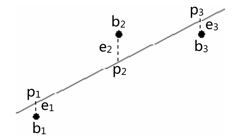
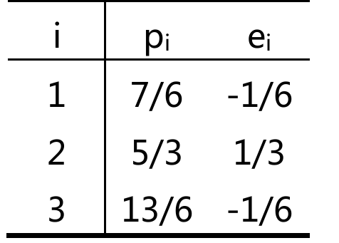
假设有三个数据点{(1,1), (2,2), (3,2)}
假设直线方程 \(b=Dt+C\)
将三个点带入方程就有\(C+D=1,C+2D=2,C+3D=2\)
$$\left[
\begin{array}{cc}
1 & 1 \\
1 & 2 \\
1 & 3 \\
\end{array}
\right]
\left[
\begin{array}{c}
C \\
D \\
\end{array}
\right]
=
\left[
\begin{array}{c}
1 \\
2 \\
2 \\
\end{array}
\right]
$$
可以发现这个Equation是无解的,但目的在于找到最优解
即方程\(A^TA\hat x =A^Tb\)的解
在这之前需要定义一个Error来判断那条直线为最优解,定义为\(||e^2||=||Ax-b||^2={e_1}^2+{e_2}^2+{e_3}^2\)
在不存在Outlier 离群值的时候是一种非常好的Regression way
\(C+Dt分别为p1,p2和p3\),它们是满足方程并最接近于b的结果
现在需要求解\(\hat x= \left[\begin{array}{c}C \D \\end{array}\right]\)和p
\(A^TA\hat x=A^Tb\)
因为\(A^T(b-A\hat x)=0\)
$$A^TA=\left[
\begin{array}{ccc}
1 & 1 & 1 \\
1 & 2 & 3 \\
\end{array}
\right]
\left[
\begin{array}{ccc}
1 & 1\\
1 & 2 \\
1 & 3\\
\end{array}
\right]
=
\left[
\begin{array}{ccc}
3 & 6\\
6 & 14\\
\end{array}
\right], A^Tb=\left[
\begin{array}{ccc}
1 & 1 & 1 \\
1 & 2 & 3 \\
\end{array}
\right]
\left[
\begin{array}{ccc}
1\\
2\\
2\\
\end{array}
\right]
=\left[
\begin{array}{cc}
5 \\
11 \\
\end{array}
\right]$$
$$\quad \text{则有}
\left[
\begin{array}{cc}
3 & 6 \\
6 & 14 \\
\end{array}
\right]
\left[
\begin{array}{c}
\hat{C} \\
\hat{D} \\
\end{array}
\right]
=
\left[
\begin{array}{c}
5 \\
11 \\
\end{array}
\right]$$
解得\(\hat C=2/3,\hat D=1/2\)
亦可以通过求Partical Derivative的方法
$$e1^2 + e2^2 + e3^2 = (C + D - 1)^2 + (C + 2D - 2)^2 + (C + 3D - 2)^2$$
$$展开结果为2 e =3C2+14D2+9-10C-22D+12CD$$
$$求偏导为12C-20+24D=0; 28D-22+12C=0。与A^TA\hat x=A^Tb相同$$
于是得到结果
可以验证p与e与A的Column Space Orthogonal
矩阵ATA
#
证明:若A的列向量线性无关时,矩阵\(A^TA\)为可逆矩阵
要证明此,假设存在x使得\(A^TAx=0\),后证明x只能是Zero Vector
第一步将灯饰两边同时乘以\(x^T\),有\(x^TA^TAx=0\)
可以重写成\((Ax)^T(Ax)=0\Rightarrow Ax=0\)
由于A的Column Vector是Linearly Independent的,所以只有\(x=0时有A^TAx=0\)
即\(A^TAx\) is invertible